

2. Load and inspect a dataset#
A query returns catalog rows. The sections below turn one row into a SpatialData object that you can analyse. It
starts with what you can learn about a dataset before you download it, because stores range from 2 MB to almost
100 GB, and a full download is often not what you need.
You will learn how to:
read the attributes of a
Datasetand list its elements without downloading anythingcheck the size of a store and choose what to fetch
load a whole store, only some elements, or a copy in a folder of your choice
find and manage the local cache
look at the tables, shapes and images of the loaded object
open the dataset on the website and in Vitessce, and know why some viewer links are hidden
The datasets here are small (under 10 MB each for what is downloaded), so the tutorial runs in a minute or two.
To run the plotting cells, install the client with the viz extra, as shown in 0. Overview: from a query to a cited cohort.
import os
import tempfile
import warnings
from pathlib import Path

import matplotlib.pyplot as plt
import numpy as np
import platformdirs
import spatialdata_plot  # noqa: F401  (adds the .pl accessor to SpatialData)
from spatialdata import get_extent

import sddb
from sddb.catalog import SITE_URL

cat = sddb.Catalog(version="2026-10-28")
work = Path(tempfile.mkdtemp())  # the files this tutorial writes go here
A Dataset and its attributes#
Catalog.dataset returns one catalog row as a Dataset. Each column of the catalog is an attribute, and a
missing value reads as None. The dataset below is a Visium section of a human pancreatic tumour, deposited in
GEO.
ds = cat.dataset("qEP9pd4LlyKeufe20000")
ds
<Dataset qEP9pd4LlyKeufe20000 technology=Visium organism=human>
{
    column: getattr(ds, column)
    for column in ["technology", "organism", "tissue", "condition", "n_obs", "n_features", "size_bytes", "license", "doi", "default_table"]
}
{'technology': 'Visium',
 'organism': 'human',
 'tissue': 'pancreas',
 'condition': 'PanIN and chronic pancreatitis in association with pancreatic ductal adenocarcinoma (PDAC)',
 'n_obs': np.int64(1142),
 'n_features': np.int64(17943),
 'size_bytes': np.int64(2577782),
 'license': 'ncbi-geo-policy',
 'doi': '10.1172/jci.insight.191595',
 'default_table': 'table'}
condition and doi come from the study, and default_table names the table that holds the main count matrix.
A cohort is a sequence of Dataset objects, so for ds in cohort and cohort[0] give the same kind of object.
Catalog.dataset also accepts the first 16 characters of the uid (the stem) and the canonical_key.
3. Cohorts and manifests explains when to use which.
Before you download#
Store sizes vary by more than four orders of magnitude. size_bytes is the size of the whole store, and most of
it is usually images:
sizes = cat.to_df()["size_bytes"]
print(f"median {sizes.median() / 1e6:.0f} MB, largest {sizes.max() / 1e9:.0f} GB, {int((sizes > 1e9).sum())} stores above 1 GB")
print(f"this dataset: {ds.size_bytes / 1e6:.1f} MB")
median 63 MB, largest 96 GB, 1172 stores above 1 GB
this dataset: 2.6 MB
Two things tell you what is inside a store without downloading it. elements() reads the store's metadata and
returns every element with its shape and data type. The sdata_repr column holds the text that print(sdata)
gives for the loaded store.
for name, info in ds.elements().items():
    print(f"{name:42s} {info['shape']} {info['dtype']}")
images/GSM8915497_PDAC04_hires_image       (3, 1215, 2000) uint8
images/GSM8915497_PDAC04_lowres_image      (3, 365, 600) uint8
shapes/GSM8915497_PDAC04                   None None
tables/table                               (1142, 17943) float32
print(ds.sdata_repr)
SpatialData object
├── Images
│     ├── 'GSM8915497_PDAC04_hires_image': DataArray[cyx] (3, 1215, 2000)
│     └── 'GSM8915497_PDAC04_lowres_image': DataArray[cyx] (3, 365, 600)
├── Shapes
│     └── 'GSM8915497_PDAC04': GeoDataFrame shape: (1142, 2) (2D shapes)
└── Tables
      └── 'table': AnnData (1142, 17943)
with coordinate systems:
    ▸ 'GSM8915497_PDAC04', with elements:
        GSM8915497_PDAC04_hires_image (Images), GSM8915497_PDAC04_lowres_image (Images), GSM8915497_PDAC04 (Shapes)
    ▸ 'GSM8915497_PDAC04_downscaled_hires', with elements:
        GSM8915497_PDAC04_hires_image (Images), GSM8915497_PDAC04 (Shapes)
    ▸ 'GSM8915497_PDAC04_downscaled_lowres', with elements:
        GSM8915497_PDAC04_lowres_image (Images), GSM8915497_PDAC04 (Shapes)
The store has two H&E images (a 2000-pixel "hires" and a 600-pixel "lowres" version, as Space Ranger writes them), one shapes element with a circle per spot, and one table with 1142 spots and 17943 genes.
Load the whole store#
to_sdata() copies the store into the local cache and opens it with spatialdata.read_zarr. A download shows a
progress bar. A later call finds the copy and opens it without downloading, so if you ran the overview, the
dataset is already in the cache and no progress bar appears.
sdata = ds.to_sdata()
sdata
SpatialData object, with associated Zarr store: /tmp/sddb-docs-cache/stores/qEP9pd4LlyKeufe20000.zarr
├── Images
│     ├── 'GSM8915497_PDAC04_hires_image': DataArray[cyx] (3, 1215, 2000)
│     └── 'GSM8915497_PDAC04_lowres_image': DataArray[cyx] (3, 365, 600)
├── Shapes
│     └── 'GSM8915497_PDAC04': GeoDataFrame shape: (1142, 2) (2D shapes)
└── Tables
      └── 'table': AnnData (1142, 17943)
with coordinate systems:
    ▸ 'GSM8915497_PDAC04', with elements:
        GSM8915497_PDAC04_hires_image (Images), GSM8915497_PDAC04_lowres_image (Images), GSM8915497_PDAC04 (Shapes)
    ▸ 'GSM8915497_PDAC04_downscaled_hires', with elements:
        GSM8915497_PDAC04_hires_image (Images), GSM8915497_PDAC04 (Shapes)
    ▸ 'GSM8915497_PDAC04_downscaled_lowres', with elements:
        GSM8915497_PDAC04_lowres_image (Images), GSM8915497_PDAC04 (Shapes)
A first look at the data#
The table is an AnnData object. X holds the counts, obs has one row per spot and var one row per gene.
In the pancreas table the gene symbols are the var_names and the Ensembl ids are in var["gene_ids"]. Other sources
store them the other way round, and the difference shows when you combine datasets (3. Cohorts and manifests).
table = sdata.tables["table"]
table
AnnData object with n_obs × n_vars = 1142 × 17943
    obs: 'in_tissue', 'array_row', 'array_col', 'spot_id', 'region'
    var: 'gene_ids', 'feature_types', 'genome'
    uns: 'spatialdata_attrs', 'spatial'
    obsm: 'spatial'
    layers: 'csc_counts'
table.var.head(3)
| gene_ids | feature_types | genome | |
|---|---|---|---|
| SAMD11 | ENSG00000187634 | Gene Expression | unknown |
| NOC2L | ENSG00000188976 | Gene Expression | unknown |
| KLHL17 | ENSG00000187961 | Gene Expression | unknown |
The table annotates the shapes element. spatialdata_attrs names the shapes element (region) and the obs
column that matches each row to a shape (instance_key):
table.uns["spatialdata_attrs"]
{'region': 'GSM8915497_PDAC04',
 'instance_key': 'spot_id',
 'region_key': 'region'}
sdata.shapes["GSM8915497_PDAC04"].head(3)
| geometry | radius | |
|---|---|---|
| spot_id | ||
| 0 | POINT (1738 1522) | 12.477101 |
| 1 | POINT (2890 1457) | 12.477101 |
| 2 | POINT (2659 1790) | 12.477101 |
Each spot is a circle with a centre and a radius. The images and shapes are placed in a common space through
coordinate systems. Space Ranger stores the image at two
resolutions, and the coordinate system ..._downscaled_hires puts the spots on top of the hires image.
The figure shows the H&E image next to two genes: COL1A1, which marks the fibrous stroma around a pancreatic
tumour, and CELA3A, an enzyme of acinar cells, the normal exocrine pancreas. The colours show log(1 + counts):
transfunc=np.log1p transforms the values only for the plot, so the counts in table stay as they are.
get_extent gives the bounding box of the spots, and crop_coord crops the empty slide around the tissue.
image = "GSM8915497_PDAC04_hires_image"
spots = "GSM8915497_PDAC04"
coordinates = "GSM8915497_PDAC04_downscaled_hires"

extent = get_extent(sdata, coordinate_system=coordinates, elements=[spots])
crop = (extent["x"][0] - 40, extent["x"][1] + 40, extent["y"][0] - 40, extent["y"][1] + 40)  # 40 pixels of margin

fig, axes = plt.subplots(1, 3, figsize=(15, 5.5))
(
    sdata
    .pl.render_images(image)
    .pl.show(
        coordinate_systems=coordinates,
        crop_coord=crop,
        ax=axes[0],
        frameon=False,
        title="H&E",
    )
)
(
    sdata
    .pl.render_images(image)
    .pl.render_shapes(spots, color=["COL1A1", "CELA3A"], table_name="table", transfunc=np.log1p)
    .pl.show(
        coordinate_systems=coordinates,
        crop_coord=crop,
        ax=list(axes[1:]),
        frameon=False,
        title=["COL1A1, log(1 + counts)", "CELA3A, log(1 + counts)"],
    )
)
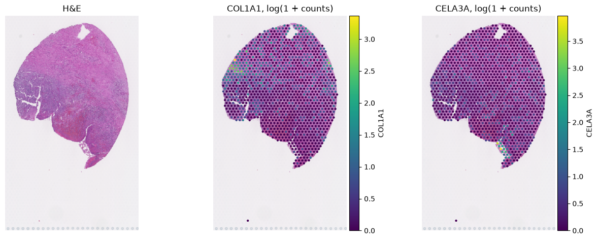
The section has few counts per spot, so most spots are dark in both panels. COL1A1 is highest along the left
edge of the section and CELA3A at the lower tip, so the two genes mark different parts of the tissue.
Load only some elements#
Most of a large store is images. If you only need the counts, elements= copies only the elements you name, as
"kind/name" paths from elements(). The client also copies the shapes or labels that a kept table annotates,
so the table keeps its link to space.
The next dataset is a Visium section from HEST. Its store is 63 MB, almost all of it a full-resolution image of
8192 by 7953 pixels. Its default_table is None, which happens for some sources, so read the table name from
elements().
hest = cat.dataset("USx288NLowiqKbV30000")
print(f"{hest.size_bytes / 1e6:.0f} MB, default_table={hest.default_table}")
for name, info in hest.elements().items():
    print(f"{name:30s} {info['shape']}")
63 MB, default_table=None
images/NCBI466_full_image      (3, 8192, 7953)
shapes/NCBI466_spots           None
tables/table                   (691, 19850)
counts_only = hest.to_sdata(elements=["tables/table"])
counts_only
UserWarning: Variable names are not unique. To make them unique, call `.var_names_make_unique`.
SpatialData object, with associated Zarr store: /tmp/sddb-docs-cache/elements/USx288NLowiqKbV30000/USx288NLowiqKbV3__abb7104aa4a2.zarr
├── Shapes
│     └── 'NCBI466_spots': GeoDataFrame shape: (691, 2) (2D shapes)
└── Tables
      └── 'table': AnnData (691, 19850)
with coordinate systems:
    ▸ 'global', with elements:
        NCBI466_spots (Shapes)
def size_on_disk(path: Path) -> float:
    """Total size of the files under ``path``, in MB."""
    return sum(f.stat().st_size for f in Path(path).rglob("*") if f.is_file()) / 1e6


print(f"copied {size_on_disk(counts_only.path):.1f} MB of {hest.size_bytes / 1e6:.0f} MB")
copied 4.3 MB of 63 MB
The copy holds the table and the spot shapes it annotates, and no image. The warning about variable names comes
from the HEST table, where two genes appear twice. 3. Cohorts and manifests shows how to_anndata handles
repeated gene names.
Keep a copy in your own folder#
Without dest, stores go to the cache. With dest, the store goes to dest/<uid>.zarr, and dest/manifest.json
records what was copied, from where, and whether the copy is whole or partial. Use dest for data that a project
depends on, so it does not live in a cache you might clear.
project = work / "data"
partial = hest.to_sdata(elements=["tables/table"], dest=project)
print(sorted(p.name for p in project.iterdir()))
print((project / "manifest.json").read_text())
['USx288NLowiqKbV30000.zarr', 'manifest.json']
{
  "generated_at": "2026-10-31T23:38:46.025989+00:00",
  "catalog_version": null,
  "entries": [
    {
      "uid": "USx288NLowiqKbV30000",
      "zarr_url": "s3://scverse-spatial-eu-central-1/.lamindb/USx288NLowiqKbV3.zarr",
      "dest": "/tmp/sddb-docs-tmp/tmp1hfpqka_/data/USx288NLowiqKbV30000.zarr",
      "size_bytes": 4335866,
      "status": "partial",
      "sha256": "3ec0e4f397cc89ec352575cf5ab2261b65bc375fcb890f4644f535219c1ed256",
      "error": null,
      "elements": [
        "tables/table"
      ]
    }
  ]
}
UserWarning: Variable names are not unique. To make them unique, call `.var_names_make_unique`.
The entry has status: "partial" and lists the elements. A later download() of a cohort with the HEST dataset into
the same folder fetches the whole store and replaces the partial copy. 3. Cohorts and manifests covers
download() and its manifest.
The cache#
The cache is a folder called sddb in your platform's user cache directory, or the folder in the environment
variable SDDB_CACHE_DIR. Set the variable before you import the client to put the cache on a larger disk.
cache = Path(os.environ.get("SDDB_CACHE_DIR") or platformdirs.user_cache_dir("sddb"))
for folder in sorted(p for p in cache.iterdir() if p.is_dir()):
    print(f"{folder.name:10s} {size_on_disk(folder):8.1f} MB")
catalog       956.6 MB
elements        4.3 MB
stores         18.0 MB
catalogholds the catalog files andcitations.bib, one per release you opened.storesholds whole stores fromto_sdata(), one<uid>.zarrper dataset.elementsholds the partial copies fromto_sdata(elements=...).
The cache is keyed by the full uid. When a dataset gets a new version, its uid changes and the client downloads the new store rather than reusing the old copy. Nothing is ever deleted for you, so remove the folder by hand when it gets large. The next call downloads what it needs again.
The website and Vitessce#
Every dataset has a page on the website, at the address built from its slug. card_url links the dataset in
Lamin, and dataset_url links the source (here the GEO series).
print(f"{SITE_URL}/datasets/{ds.slug}/")
print(ds.card_url)
print(ds.dataset_url)
https://spatialdata-db-web.pages.dev/datasets/visium-spatial-gene-expression-pancreas-qep9pd4llykeufe20000/
https://lamin.ai/scverse/spatialdata-db/artifact/qEP9pd4LlyKeufe20000
https://www.ncbi.nlm.nih.gov/geo/query/acc.cgi?acc=GSE294669
viewer_url() returns a link that opens the dataset in Vitessce, a viewer that runs in the browser. The link
contains the whole viewer configuration, so it is long. view() opens it in your browser, and
view_interactive() shows it inside a notebook. Both need the viz extra.
url = ds.viewer_url()
print(url[:80] + "...", f"({len(url)} characters)")
https://vitessce.io#?edit=false&url=data:,%257B%2522version%2522%253A%2520%25221... (8963 characters)
In the 2026-10-28 release, 333 of the 5937 viewer links load the store of another dataset, because of an error
in the catalog. The client checks every link against the dataset's own store, as the website does. For a link
that does not match, viewer_url() warns and returns None, and view() raises a ValueError. The viewer link
of a small Xenium kidney section, NHyd5DFysygNrkdu0000, is one of them:
kidney = cat.dataset("NHyd5DFysygNrkdu0000")
with warnings.catch_warnings(record=True) as caught:
    warnings.simplefilter("always")
    print(kidney.viewer_url())
print(caught[0].message)
None
the viewer link for NHyd5DFysygNrkdu0000 loads another dataset's store; it is hidden until the catalog is fixed
Counting the hidden links over the whole catalog gives the 333. The warnings are switched off here, because there would be one per hidden link.
with warnings.catch_warnings():
    warnings.simplefilter("ignore")
    hidden = [d.uid for d in cat.query() if d.vitessce_url and d.viewer_url() is None]
print(len(hidden), "viewer links hidden")
333 viewer links hidden
Summary#
Datasetattributes,elements()andsdata_reprdescribe a dataset without a download. Checksize_bytesfirst.to_sdata()caches the whole store,elements=copies only what you name, anddest=keeps a copy with a manifest in a folder of your choice.The cache lives in
SDDB_CACHE_DIRor the user cache directory, keyed by full uid.viewer_url()returnsNonewith a warning when a link would open another dataset.
Next: 3. Cohorts and manifests, which works with many datasets at once and makes the selection reproducible.